tensor: multi-index array of (real) numbers (typically \(\ge 3\) indices)

mode: index position
3-tensor over \({\mathbb{R}}^d\)

\(T\) is \(d^3\)-dimensional, each mode is \(d\)-dimensional
Kronecker/tensor product: combine lower-order tensors to higher-order ones (called product tensors)
for example, \(\displaystyle T = \sum_{i,j,k\in [d]} T_{ijk} \cdot e_i\otimes e_j \otimes e_k\) (coordinate basis \({\left\{ e_i \right\}}_{i\in [d]}\))
natural shape of data
- moments of high-dimensional distributions, \(M_3 = {\mathbb{E}}_{D(x)} x^{\otimes 3}\)
- multivariate polynomials, \(T(x)=\sum_{i,j,k} T_{i,j,k} \cdot x_i x_j x_k\)
- quantum states of multi-part systems, \(|\psi \rangle \in A \otimes B \otimes C\)
- basic data structure in machine-learning frameworks like tensorflow, torch, theano
“tensors are the new matrices”
tie together wide ranges of disciplines
basic problem about tensors:
tensor decomposition: given 3-tensor \(T\), decompose \(T\) as sum of as few product tensors as possible, so that
graphical representation:

widely studied, e.g., in signal processing and machine learning
intuition: explain data in simplest way possible
powerful general primitive for unsupervised learning
efficient unsupervised learning via tensor decomposition
- blind-source separation, independent component analysis [Comon’94, Belouchrani-Abed-Meraim-Cardoso-Moulines’97]
- mixtures of (many) Gaussians [Hsu-Kakade’13, Ge-Huang-Kakade’15]
- dictionary learning / sparse coding [Barak-Kelner-S.’15]
- topic modeling (latent dirichlet allocation)
[Anandkumar-Ge-Hsu-Kakade-Telgarsky’14]
- overlapping community detection [Anandkumar-Ge-Hsu-Kakade’14]
- phylogenetic tree / hidden Markov model [Chang’96, Mossel-Roch’05]
(some details later)
key advantage over low-rank matrix factorization:
- rotation problem: matrix factorizations never unique
(unless we add strong restrictions like orthogonality or nonnegativity)
\[ \textstyle \sum_{i=1}^r a_i b_i^T = A \cdot B^T = (A R) \cdot (B R^{-1})^T \](two different factorizations for same matrix)
- in contrast: tensor decomposition often\({}^\ast\) unique
\({}^\ast\) under mild assumptions on the factorization (details later)
challenges: beyond worst-case complexity
tensor decomposition is NP-hard in the worst case [Håstad]
\(\leadsto\) cannot hope for same algorithmic theory as for matrices
but: can still hope for strong provable guarantees (like for approximation algorithms, compressed sensing, or matrix completion)
tractability appears to go hand in hand with uniqueness
with sos [Barak-Kelner-S.’15, Hopkins-Schramm-Shi-S.’16, Ma-Shi-S.’16]
algorithmic framework for efficient tensor decomposition
- unifies and extends many previous approaches
- based on convex relaxations for polynomial optimization (namely sum-of-squares)
- achieves strongest known provable guarantees
- connection to constructive proofs
- also allows for fast practical algorithms
concrete consequences
- first efficient algorithms for “overcomplete” 3-tensors
(rank of tensor \(\gg\) dimension of modes)
- robust enough to enable new applications (e.g., dictionary learning / sparse coding [BKS’15] and Bayes nets [Arora-Ge-Ma-Risteski’16])
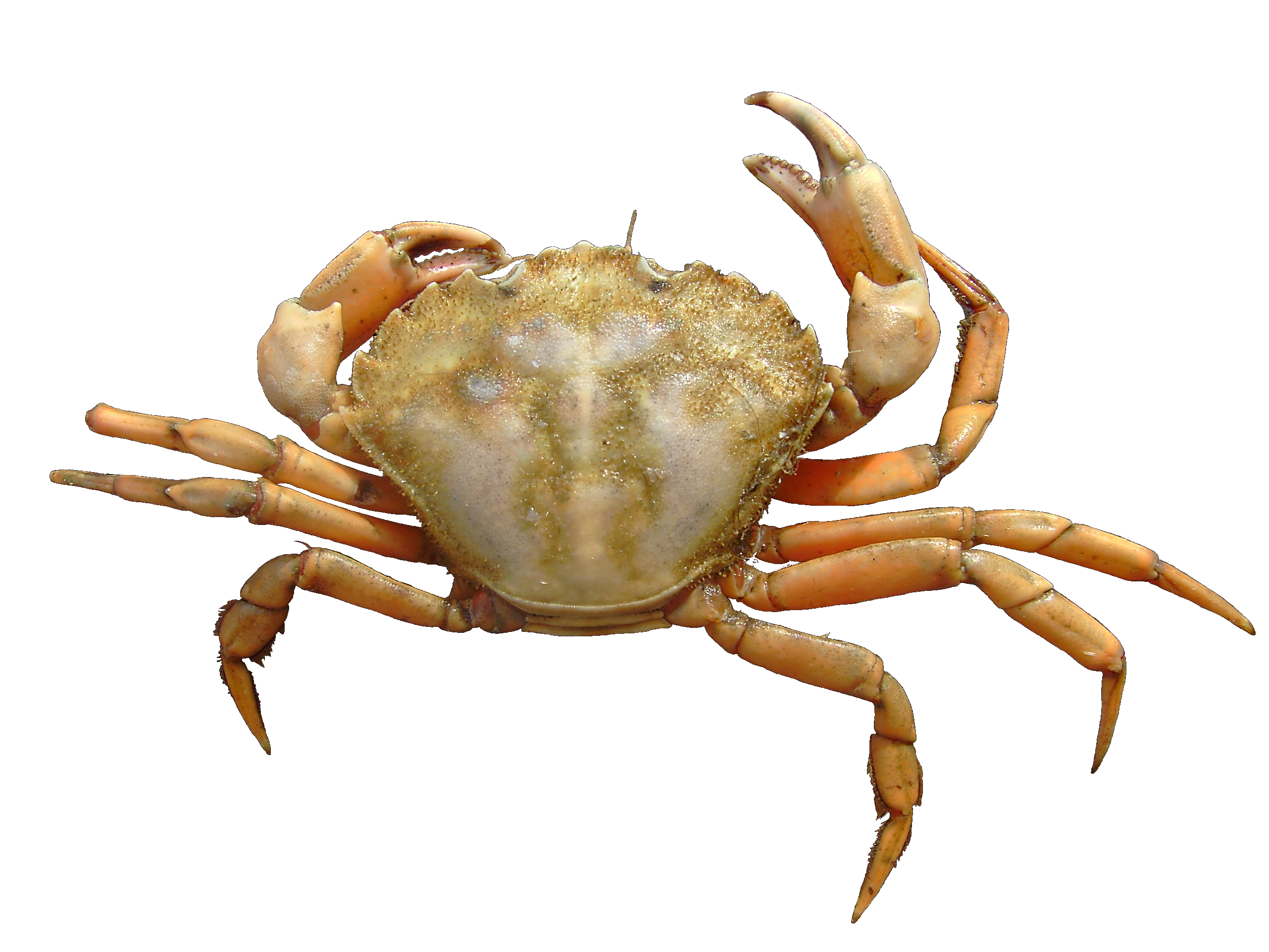
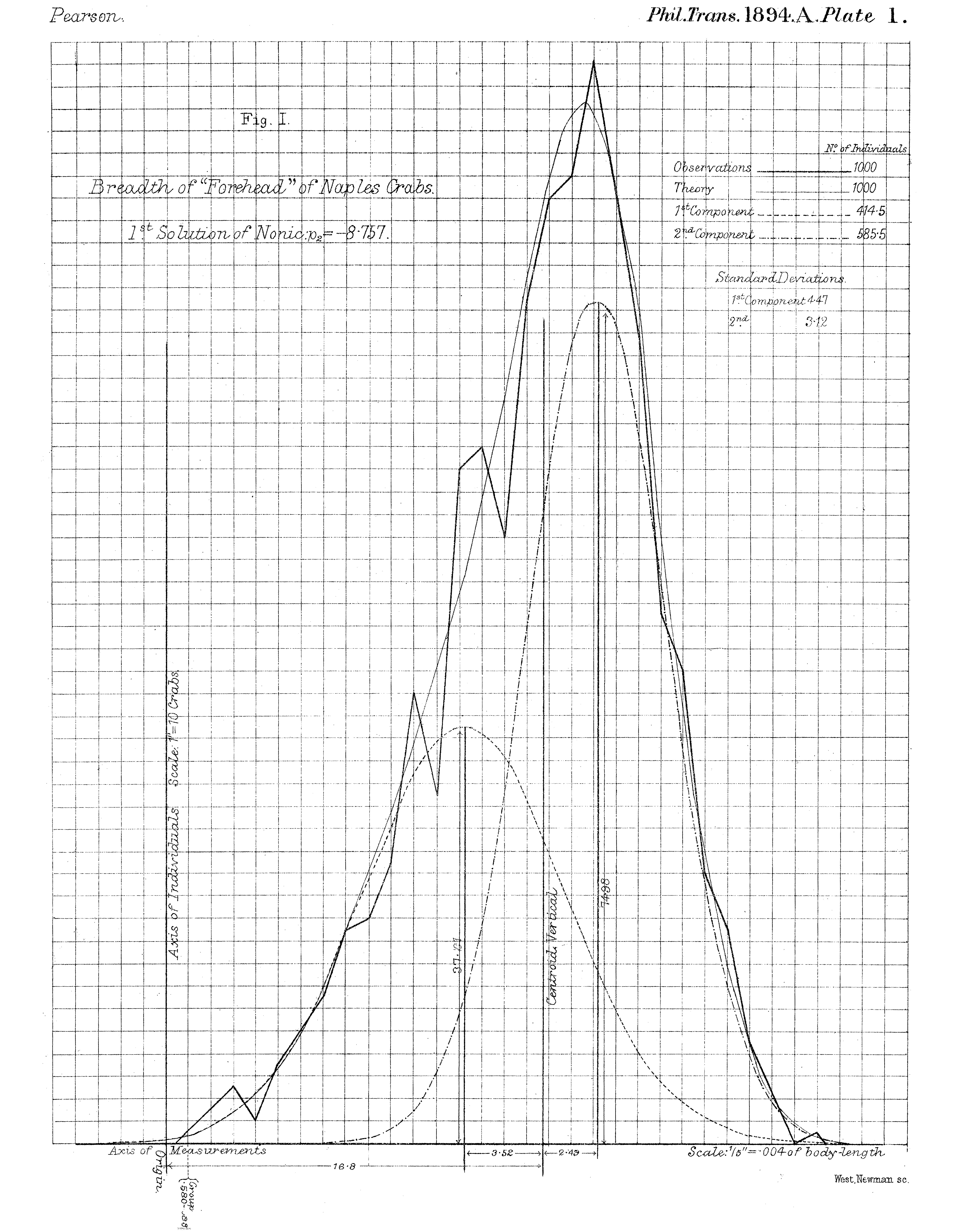
Karl Pearson (1894) and the Naples Crabs
learning mixtures of Gaussians (GMM)
soft clustering problem (overlapping clusters)
unknown: cluster centers \(a_1,\ldots,a_n\in {\mathbb{R}}^d\)
given: iid samples \(x_1,\ldots,x_m\) from mixture of \({\{ N(a_i,{\mathrm{Id}}_d) \}}_{i\in [n]}\):
\(x_j = a_i + g\) for random idx \(i\in [n]\) and Gaussian \(g\sim N(0,{\mathrm{Id}})\)
find: set of vectors \(\approx{\{ a_1,\ldots,a_n \}}\)
learning GMMs with tensor decomposition
unknown: cluster centers \(a_1,\ldots,a_n\in {\mathbb{R}}^d\)
given: iid samples \(x_1,\ldots,x_m\) from mixture of \({\{ N(a_i,{\mathrm{Id}}_d) \}}_{i\in [n]}\)
find: set of vectors \(\approx{\{ a_1,\ldots,a_n \}}\)
also works for non-uniform mixing weights and covariance matrices
- compute empirical moments \({\widetilde M}_k = \tfrac 1m \sum_{i=1}^m x_i^{\otimes k}\) for \(k\le 3\)
- estimate 3-tensor \(\sum_{i=1}^n a_i^{\otimes 3}\) by polynomial \(P({\widetilde M}_1,{\widetilde M}_2,{\widetilde M}_3)\)
- recover \(a_1,\ldots,a_n\) by decomposing this tensor (robustly)
how to choose the polynomial \(P\)? (cannot depend on \(a_1,\ldots,a_n\))
\(\exists\) deg-3 polynomial \(P\) such that for actual moments \({\mathcal M}_k={\mathbb{E}}x^{\otimes k}\)
\(\leadsto\) for \(m=n^{O(1)}\) samples, we have \({\mathcal M}_k \approx {\widetilde M}_k\) and
thus \(P({\widetilde M}_3,{\widetilde M}_1) \approx P({\mathcal M}_3,{\mathcal M}_1)\) as desired
sparse coding / dictionary learning
what’s the “right” basis / representation for my data?
Pixel basis, Fourier basis, Wavelet basis, Eigen basis, …
desirable property of representations: sparsity
unsupervised learning of sparse representations for data:
given: data points \(x_1,\ldots,x_m\in {\mathbb{R}}^d\)
find: sparse vectors \(y_1,\ldots,y_m\in {\mathbb{R}}^n\) and matrix \(A\in {\mathbb{R}}^{d \times n}\) s.t.
vectors \(y_1,\ldots,y_m\) are sparse representations of \(x_1,\ldots,x_m\) and
matrix \(A\) is dictionary from sparse to original representation
originally proposed as model for visual cortex [Olshausen, Field’96]
extensively studied in different disciplines
important regime: \(n \gg d\) (“overcomplete” representation)
example: sparse dictionaries for natural image patches
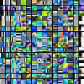
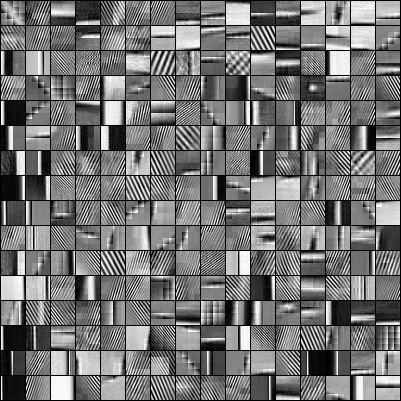 [Mairal, Sapiro, Elad’07]
example application: computer vision
use sparse dictionary for inpainting (“healing” images)
[Mairal, Bach, Ponce, Sapiro’09]


many other applications for sparse dictionaries
(e.g., reduce required amount of labeled data)
algorithms for dictionary learning
given: data points \(x_1,\ldots,x_m\in {\mathbb{R}}^d\)
find: sparse \(y_1,\ldots,y_m\in {\mathbb{R}}^n\) and \(A\in {\mathbb{R}}^{d \times n}\) s.t. \(x_j = A y_j\)
natural formulations as optimization problem are NP-hard
alternating minimization works well but no strong guarantees
recent alg’s with provable guarantees [Spielman-Wang-Wright’12; Agarwal-Anandkumar-Jain-Netrapalli-Tandon’14; Arora-Ge-Moitra’14]
works propose generative models (planted distributions)
common barrier for techniques: require sparsity \(\le \sqrt n\)
with SOS: [Barak-Kelner-S.’15; Ma-Shi-S.’16] only require sparsity \(\ll n\)
(based on new tensor decomposition algorithms)
generative model for dictionary learning:
dictionary: col’s of \(A\) separated unit vectors; \(\sigma_\max(A)\le O(1)\)
sparse representations:
\(y_1,\ldots,y_m\) iid from “nice” but unknown distribution over \(\tau\cdot n\)-sparse vectors
connection to tensor decomposition: 4-th moment of distr’n \({\{ x \}}\) satisfies for \(A=(a_1,\ldots,a_n)\)
\(\leadsto\) can recover \(A\) by decomposing empirical mom’t \(\tfrac 1 m \sum_{j=1}^m x_j^{\otimes 4}\)
crucial: tensor decomposition robust against systematic error \(E\)
tensor decomposition as moment problem:
unknown: finite set of vectors \({\mathcal A}={\{ a_1,\ldots,a_n \}}\subseteq {\mathbb{R}}^d\)
given: low-deg. moments \({\mathcal M}_1,\ldots,{\mathcal M}_k\) of unif’m distr’n over \({\mathcal A}\)
find: set of vectors close to \({\mathcal A}\)
how many moments do we need
(under some assumptions on the vectors)
to recover the vectors efficiently and robustly?
main open questions:
• when are 3 moments enough for \(n \gg d\) vectors? (overcomplete)
• how robust against error in input tensor?
concrete results: [BKS’15,MSS’16] first polynomial-time algorithms
… for overcomplete 3-tensors (under mild assumption on vectors)
… robust against spectral norm error (same order as signal)
high-level approach
“dream up” higher-degree moments from given moments
using sum-of-squares convex relaxations
apply classical decomposition alg’s to “dream moments” (analogous to rounding algorithm)
“dream moments” behave like real moments
w.r.t. restricted but powerful proof system
new algorithms require less data and are more robust
Jennrich’s random contraction algorithm (1970s)
unknown: orthonormal vectors \(a_1,\ldots,a_n\in {\mathbb{R}}^d\)
given: 3-tensor \(T=\sum_{i=1}^n a_i^{\otimes 3}\in ({\mathbb{R}}^d)^{\otimes 3}\)
find: vectors \(a_1,\ldots,a_n\)
corollary 1: can recover linearly independent vectors from their 2nd and 3rd moments (orthonormalize vectors using 2nd moment)
corollary 2: if vectors \(a_1^{\otimes k},\ldots,a_n^{\otimes k}\) are linearly independent can recover \(a_1,\ldots,a_n\) from \(2k+1\)-st moment
random contraction: bilinear map from \(d\)-dim Gaussian vector \(g\) and \(d\times d \times d\)-dim tensor \(T\) to \(d\times d\)-dim matrix,
algorithm: output eigenvectors of random contraction of \(T\)
\(\leadsto\) w.h.p all eigenvalues \({\langle g,a_i \rangle}\) distinct and eigenbasis unique
how robust is this algorithm? (later: new analysis using matrix bernstein)
approach for overcomplete 3-tensors
let \(a_1,\ldots,a_n\in {\mathbb{R}}^d\) be unit vectors with \(n\gg d\) (Jennrich’s alg. fails)
- lift 3rd moment of \({\{ a_i \}}\) to 6th moment of \({\{ a_i \}}\)
- apply classical random contraction to lifted moment (viewed as 3rd moment of \({\{ a_i^{\otimes 2} \}}\))
second step works under mild assumptions on \({\{ a_i \}}\)
(tensored vectors \({\{ a_i^{\otimes 2} \}}\) close to orthogonal)
how can we lift moments (approximately)?
first attempt: find distribution \(D\) over unit vectors with matching 3rd moment and output 6th moment of \(D\)
\(\leadsto\) lifted 6th moment close to correct under mild assumptions on \({\{ a_i \}}\)

underlying reason: \({\{ a_i \}}\) approx. global maximizers of \(f(x)=\sum_{i=1}^n {\langle a_i,x \rangle}^3\) over unit sphere
- distr’n with matching moments NP-hard to find in worst-case 🙁
\(\leadsto\) search over “pseudo-distributions” instead ☺ (general theme)
- random contraction algorithm not robust enough 🙁
\(\leadsto\) reduce error by maximizing entropy of \(D\) and use new analysis of alg using matrix concentration bounds ☺
robust analysis of Jennrich’s algorithm
let \({\{ b_i \}}\) be (close to) orthonormal vectors (\(b_i=a_i^{\otimes 2}\) in previous slide)
theorem: [MSS’16] if \(E=T-\sum_{i=1}^n b_i^{\otimes 3}\) is symm. and has small spectral norm (as \(d^2\times d\) matrix), then with probability \(\ge 1/n^{O(1)}\) top eigenvector of \(\mathrm{contraction}(T,g)\) is close to \(b_i\)
\(\mathrm{contr'n}(T,g)=\underbrace{\mathrm{contr'n}(\sum_i b_i^{\otimes 3},g)}_{\text{no noise}} + \underbrace{\mathrm{contr'n}(E,g)}_{\color{red}{\text{want: small spectral norm}}}\)
key insight: \(\mathrm{contr'n}(E,g)\) is linear matrix polynomial in Gaussian variables \(\leadsto\) great bounds for spectral norms [Oliveira;Tropp]
lemma:
this analysis robust enough to apply to lifted moments 🙂
probability meets computational complexity
pseudo-distributions:
computationally efficient relaxation of probability distributions
(here: discrete distributions over unit sphere)
- “low-complexity” events always have nonneg’ve probability 🙂
- “high-complexity” events may have “negative probability” 🙁
definition: level-\(\ell\) pseudo-distr’n over sphere \(\mathbb S^{d-1}\subseteq {\mathbb{R}}^d\)
- finitely supported function \(D{\colon}\mathbb S^{d-1}\to {\mathbb{R}}\)
- \(\sum_{x} D(x)=1\) (sum is over support of \(D\))
- \(\sum_x D(x) \cdot f(x)^2 \ge 0\) whenever \(\deg f \le \ell\)
level-\(\infty\) pseudo-distr’n is classical probability distr’n
moments of pseudo-distr’n (will use them for matching and lifting)
theorem: [Shor’85,Parrilo’00,Lasserre’00] set of moments of level-\(\ell\) pseudo-distr’n have \(n^{O(\ell)}\) time separation oracle
key step: check \(M_{2k}(D)\succeq 0\) for \(k\le \ell\) (as \(d^k\times d^k\) matrix)
most alg’s based on convex relaxations captured by pseudo-distr’n
sum-of-squares proof system
to what extent behave pseudo-distributions like classical distr’s?
def’n: deg-\(\ell\) SOS proof of \({\{ \forall x\in \mathbb S^{d-1}.~f(x)\ge g(x) \}}\)
functions \(h_1,\ldots,h_r\) with \(\deg h_j\le \ell\)
many classical ineq’s have SOS proofs: Cauchy–Schwarz, Hölder, …
capture properties of pseudo-distr’s (all properties by duality)
lemma: if \({\{ f\ge g \}}\) has deg-\(\ell\) SOS proof, then \(\sum_x D(x)\cdot f(x)\ge \sum_xD(x)\cdot g(x)\) for all level-\(\ell\) pseudo-distr’s \(D\)
moment matching with pseudo-distr’s
reason that moment matching works for classical distributions:
(related to notion of identifiability)
fact: \({\{ a_i \}}\approx\) global maximizers of \(x \mapsto \sum_{i=1}^n {\langle a_i,x \rangle}^3\) over sphere
want: moment matching works even for pseudo-distributions
to show: low-degree SOS proof for above fact
SOS proof of identifiability: \(\exists\) low-deg. polynomials \(g_1,\ldots,g_r\) (depending on \({\{ a_i \}}\)) such that \(\forall\) unit vectors \(x\in{\mathbb{R}}^d\),
where are we now?
we saw: general algorithmic scheme based on lifting and matching moments for tensor decomposition and applications (e.g., learning Gaussian mixtures and sparse dictionaries)
pros:
- strongest known guarantees for many input distributions
- polynomial running time
cons:
- working with lifted moment expensive (\(d^6\)-dimensional)
- getting lifted moments very expensive (large semidefinite program)
good in theory, but not useful in practice 🙁
will see: simple general strategy to extract fast practical algorithms from scheme with similar guarantees 🙂
concrete sample result: decompose \(d^3\)-dimensional overcomplete \(3\)-tensor in \(d^{1+\omega}\) time where \(\omega\le 2.373\) is fast matrix multip’n exponent (close to linear time in input size)
general strategy
starting point: lift moments in simpler way instead of matching moments with pseudo-distributions
why could this work?
pseudo-distributions need to fool all low-deg SOS proofs
we only need to fool Jennrich’s random contraction algorithm
approach: lift mom’s by explicit low-deg polynomial \(P\) in input tensor (choice of \(P\) informed by SOS proofs that appear in analysis)
crucial: can avoid higher tensors by exploiting tensor structure of \(P\) to “unroll” Jennrich’s algorithm
tensor decomposition in tensorflow™
our resulting algorithm has simple “one-line” implementation
# [d,d,d]-dimensional 3-tensor
T = tf.constant(...)

# [d]-dimensional random vector
g = tf.constant(tf.random_normal([d]))

# [d,d]-dimensional random matrix
X = tf.constant(tf.random_normal([d,d]))

# iterations
for i in range(iter_num):
    X = tf.einsum('abi,cdj,ijk,k,bd->ac',T,T,T,g,X)

session.run(X)
(update \(X\) by evaluating 5-linear form in \(T\), \(T\), \(T\), \(g\), and \(X\))
summary
two-step algorithm design paradigm based on pseudo-distr’s:
- design algorithm based on (false) assumption that we can optimize over moments of distributions
- get poly-time algorithm by showing that pseudo-distr’s have same properties
first step often easier than coming up with efficient algorithm
for second step, large toolbox is emerging (reusable analyses)
for machine learning problems, search over moments gives systematic way to reduce data requirements
sos proof of identifiability
unit vectors \(a_1,\ldots,a_n\in {\mathbb{R}}^d\) with
\(\max_{i\neq j} {\lvert {\langle a_i,a_j \rangle} \rvert}\le \rho\)
and \(\sum_i {a_i {a_i}^\intercal} \preceq \sigma\cdot {\mathrm{Id}}\)
and \(\rho \sigma^2 \le o(1)\)
\(\exists\) low-deg. polynomials \(g_1,\ldots,g_r\) (depending on \({\{ a_i \}}\)) such that
\(\forall\) unit vectors \(x\in{\mathbb{R}}^d\),
proof strategy:
- find “simple regular proof” of inequality
- check that all steps are “low-deg SOS equalities”
\(\color{red}{\sum_i {\langle a_i,x \rangle}^3}\)
\(\quad ={\left\langle x, \sum_i {\langle a_i,x \rangle}^2 a_i\right \rangle}\)
\(\quad \le \tfrac 12 {\| x \|}^2 + \tfrac12 {\left\| \sum_i {\langle a_i,x \rangle}^2 a_i \right\|}^2\)
\(\quad = \quad\ldots \quad + \tfrac12 \sum_{i,j} {\langle a_i,a_j \rangle}\cdot {\langle a_i,x \rangle}^2 {\langle a_j,x \rangle}^2\)
\(\quad \le \quad\ldots \quad + \tfrac12 \color{red}{\sum_i {\langle a_i,x \rangle}^4} + \tfrac 12 \sum_{i\neq j} \rho\cdot {\langle a_i,x \rangle}^2 {\langle a_j,x \rangle}^2\)
\(\quad \le \quad\ldots \quad +\quad \quad \ldots \quad \quad + \tfrac 12 \sum_{i\neq j} \rho \sigma^2 \cdot {\| x \|}^2\)
easy to check: each inequality here is actually an equality up to sums of low-degree squares
recall: tensorflow™ implementation
# [d,d,d]-dimensional 3-tensor
T = tf.constant(...)

# [d]-dimensional random vector
g = tf.constant(tf.random_normal([d]))

# [d,d]-dimensional random matrix
X = tf.constant(tf.random_normal([d,d]))

# power iteration for linear operator on [d,d]-dim matrices
for i in range(iter_num):
    X = tf.einsum('abi,cdj,ijk,k,bd->ac',T,T,T,g,X)

session.run(X)
(update \(X\) by evaluating 5-linear form in \(T\), \(T\), \(T\), \(g\), and \(X\))
unit vectors \(a_1,\ldots,a_n\in {\mathbb{R}}^d\) with
\(\max_{i\neq j} {\lvert {\langle a_i,a_j \rangle} \rvert}\le \rho\)
and \(\sum_i {a_i {a_i}^\intercal} \preceq \sigma\cdot {\mathrm{Id}}\)
and \(\rho \sigma^{10} \le o(1)\)
key theorem: for Gaussian vector \(g\in {\mathbb{R}}^d\), following matrix has top eigenvector close to \(a_i\) with prob \(1/n^{O(1)}\) [Schramm-S.’17+]
above matrix \(M\) is explicit polynomial in \(T=\sum_i a_i^{\otimes 3}\) and \(g\) and
has \(O(d^{1+\omega})\)-time matrix-vector mult’n alg’m given \(T\) and \(g\)
\(\leadsto\) close to linear time alg. to find one \(a_i\) given \(T\)
by matrix bernstein, enough to bound spectral norm of
key step: bound contribution of terms with \(i\neq j\)
let \(x\in {\mathbb{R}}^{d^3},y\in {\mathbb{R}}^{d^2}\) be unit vectors
claim: \(\sum_{i\neq j} \sum_k {\langle a_i,a_k \rangle}{\langle a_j,a_k \rangle} \cdot {\langle a_i\otimes a_j\otimes a_k,x \rangle} {\langle a_i \otimes a_j,y \rangle} \le O(\rho\cdot \sigma^{10})^{1/2}\)
after Cauchy–Schwarz: to show \(\sum_k {\langle a_i,a_k \rangle}^2{\langle a_j,a_k \rangle}^2\le \rho \sigma\) for \(i\neq j\)
\(\sum_k {\langle a_i,a_k \rangle}^2{\langle a_j,a_k \rangle}^2\)
\(\le \sum_k \rho\cdot {\lvert {\langle a_i,a_k \rangle} \rvert}{\lvert {\langle a_j,a_k \rangle} \rvert}\)
\(\le \rho\cdot (\sum_k {{\langle a_i,a_k \rangle}}^2)^{1/2}\cdot (\sum_k{{\langle a_j,a_k \rangle}})^{1/2}\)
\(\le \rho \sigma\)